
Workflows
On a Mac, use ⌘ in place of Ctrl in the shortcuts below.
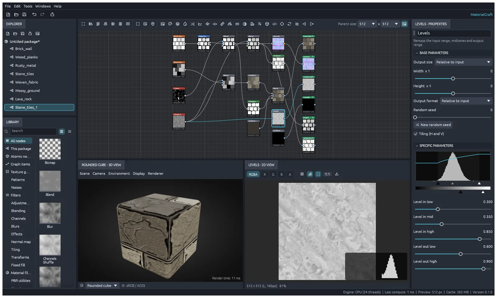
The panels
Section titled “The panels”| Panel | What it’s for |
|---|---|
| Explorer | The open package and its graphs. Click a graph to open it |
| Library | Every node you can add. Search it, or drag a node onto the graph |
| Graph | Where you build the material |
| Properties | The settings of the selected node, or of the graph |
| 2D View | One node’s result as a flat image |
| 3D View | The whole material on a shape or a model |
| Console | Messages, warnings and errors |
| History | Your recent changes |
Open or close panels from the Windows menu. Windows › Reset layout puts them back where they started.
Packages and graphs
Section titled “Packages and graphs”A package is one .sbs file. It can hold several graphs, plus the images they use.
- File › New › Graph… adds a graph to the open package.
- File › New › Function Graph… adds a function graph: a graph of math operations, saved in the package.
- File › New › Empty package starts again with an empty package.
- File › Open… opens an .sbs package, or a .mcmat material.
Build the graph
Section titled “Build the graph”- Point at the graph and press Space or Tab to search for a node. Right-click the graph for Add node and more.
- Drag from an output port to an input port to connect two nodes.
- Double-click a node to show it in the 2D View.
- Select nodes and choose Tools › Create graph from selection to turn them into a graph of their own.
- Right-click the graph to add a comment, a frame, or a navigation pin. F2 and Shift+F2 jump between pins.
- Tools › Snap to grid turns snapping on or off.
| To | Do this |
|---|---|
| Zoom | Scroll the wheel |
| Pan | Middle-drag, or Alt+drag |
| Frame everything, or the selection | F |
| Duplicate | Ctrl+D |
| Copy, cut, paste | Ctrl+C, Ctrl+X, Ctrl+V |
| Select every node | Ctrl+A |
| Delete | Delete |
| Delete a node and join its wires back up | Backspace |
| Turn the selected nodes off | Shift+D |
| Undo, redo | Ctrl+Z, Ctrl+Y |
Edit wires
Section titled “Edit wires”- Click a wire to select it. Shift+click or Ctrl+click selects more.
- Press Delete to remove the selected wires.
- Select two or more wires into a node and press X to swap where they come from. On a Blend node, this swaps the foreground and background.
- Drag a wire to pull a reroute dot out of it. Double-click a wire to drop a dot there.
- Right-click a wire for Insert reroute dot and the other wire commands.
Use graph inputs and outputs
Section titled “Use graph inputs and outputs”- Output nodes are what the graph makes. Give each a usage, such as base color, normal or roughness. The 3D View and the export use them.
- Input color, Input grayscale and Input value nodes are inputs of the graph. Use them to feed in an image or a value from outside.
Expose a parameter as a graph input
Section titled “Expose a parameter as a graph input”An exposed parameter becomes a slider or color on the graph itself, so you can tune the material without opening its nodes.
- Right-click a node’s parameter in Properties and choose Expose as graph input.
- Clear the selection to show the graph’s own Properties. The parameter is listed under Input parameters. This is also where you find Random seed and the graph’s Attributes: category, description, author and tags.
- To keep a look, type a Preset name and choose Save preset. The Presets list applies it again later. Delete preset removes the one named in the field.
To delete an input, use the x beside it. To feed an exposed input into another node’s parameter, right-click that parameter and choose Bind to input.
The command-line tool sets exposed inputs with --set, as shown in Use it with an AI assistant.
Write a function
Section titled “Write a function”Pixel processor computes every pixel of its image with a function. Value processor computes one value with a function.
Select the node, then choose Edit function graph… in Properties. In the function editor you add operations, set constants, wire them up and pick the result.
Make a pattern with an FX-Map
Section titled “Make a pattern with an FX-Map”An FX-Map node builds an image by placing and repeating shapes.
- Select the FX-Map node and press Ctrl+E (Edit › Edit node graph), or right-click it and choose Edit graph.
- Inside, add Quadrant, Switch, Iterate and Dot nodes. Wire them from bottom ports to top ports.
- Right-click a node and choose Set as root to make it the start of the pattern.
- Press Alt+Left (Edit › Parent graph) to go back to the main graph.
Adjust levels
Section titled “Adjust levels”Select a Levels node. Properties shows a histogram of the node’s input, with the levels curve over it. Drag the handles under the histogram to set the input range and midtones, and the handles under the gray bar to set the output range. The sliders below give exact values.
Use images
Section titled “Use images”Choose File › Import bitmap… to add an image to the package. MaterialCraft reads SVG, PNG, JPEG, TGA, TIFF, BMP, WebP, OpenEXR and Radiance HDR. Use it in the graph with a Bitmap or SVG node. File › Reload resources reads the files again after you change them.
Preview your material
Section titled “Preview your material”In the 2D View, show one channel (R, G, B or A) or all of them, turn on a histogram, or tile the image three by three to check its edges. Save image… saves what you see as PNG, OpenEXR or TGA.
The 3D View has its own menus:
- Scene: pick a shape, load your own OBJ, glTF or GLB model with Load mesh…, or Reset scene.
- Camera, Environment, Display and Renderer: the view, the lighting, and options such as tiling, height depth, transparency and Flip normal map Y (DirectX).
Shift+drag in the 3D View turns the lighting. Tools › View outputs in 3D view puts the graph’s outputs on the 3D model.
While you edit, previews are computed at a smaller size to stay fast. Change it in Tools › Preview size.
Export
Section titled “Export”- File › Export outputs… (Ctrl+Shift+E) writes every output of the graph as an image. Pick the Folder, Format, Bit depth, Resolution (up to 8192 pixels) and the File names pattern.
- File › Export material… writes a portable .mcmat file with the maps and the graph together.
Preferences
Section titled “Preferences”Choose Edit › Preferences… to set the language (English or Arabic), brightness, accent color, interface scale, how often to autosave, the preview size while editing, node thumbnails, and how the 3D view pans.
Help › Shortcuts list… lists every shortcut.
Use it with an AI assistant
Section titled “Use it with an AI assistant”MaterialCraft’s command-line tool, materialcraft-cli, has an MCP server, so Claude and other AI assistants can build graphs, set parameters and export maps. Give it the folders it may read and write:
claude mcp add materialcraft -- materialcraft-cli mcp --read-root . --write-root .To see its changes live, start the app with materialcraft --control 7878, then connect with materialcraft-cli mcp --bridge 7878.
The tool also works on its own. Run materialcraft-cli --help to see what it can do, for example:
materialcraft-cli new pbr my-material.sbs --size 2048materialcraft-cli export my-material.sbs textures --format png --depth 16materialcraft-cli render my-material.sbs preview.png --scene sphereMore commands
Section titled “More commands”| Command | What it does |
|---|---|
new <template> <out.sbs> |
Makes a package. The templates are empty, pbr and atomics |
info <package> |
Lists the graphs, nodes and outputs |
nodes |
Lists the node library. Narrow it with --filter or --category |
cook <package> |
Computes a graph and reports the time and errors for each node |
run <package> <command-id> |
Runs one command. Add -o out.sbs to save the result |
batch <script.json> |
Runs a list of commands from a file |
serve |
Takes commands as JSON lines, on stdio or on a local port |
cook, export and render accept --set to give an exposed graph input a value first. Use JSON for the value:
materialcraft-cli export my-material.sbs textures --set roughness=0.4 --set tint="#aa7744"render also takes --scene (rounded_cube, cube, sphere, cylinder, plane, torus or material_ball), --tiling, --view 2d --node <id> to render one node, and --hq for a finer, lit render. Where a command wants a package, sample stands for the built-in Atomic sample.
Connect to a running app
Section titled “Connect to a running app”The control port needs a token, so other programs on your computer can’t drive the app. materialcraft --control 7878 writes one to a file in your temp folder, and materialcraft-cli mcp --bridge 7878 reads it. To use your own, set MATERIALCRAFT_CONTROL_TOKEN (16 to 1024 characters) before you start the app, or pass the token with --token.